School · February – June 2026

MicroGrid laboratory

Master thesis at Icam Toulouse. Three of us spent a semester building CHESS.lab: a research and teaching platform for AC microgrids. Rooftop plant, indoor bays, sensing, and a Simulink model of the inner loops.

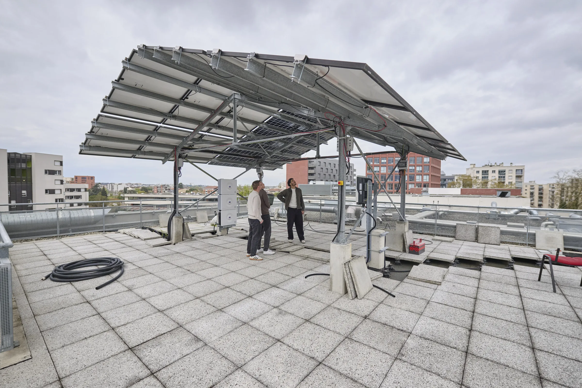
The lab has to serve both teaching and research. The question we worked against: how do you build an experimental platform that is modular, reproducible and cheap enough, and still lets you characterise the dynamics of a microgrid with real sources, then test how stable and resilient it is under a disturbance?

Three objectives sat under that: stand up the lab, bring the rooftop renewables onto the indoor emulator (not done yet), and emulate the usual low-voltage distribution topologies (ring, mesh, radial) on a board you can rewire.

I did this with Marween Jaouad and Cyril Portoles, under Allal Bouzid.

Two platforms, one lab

CHESS.lab is split in two, on purpose. Outside, on the roof: 12 kW of PV, a 9.6 kWh Li-ion stack, two vertical-axis wind turbines, and the cabinets that land those sources on the building network. Inside: four 19-inch bays and a wall of distribution topologies. The indoor bays are the emulator. The roof is the real plant. The two are not connected yet; tying them together is a later objective.

Roof

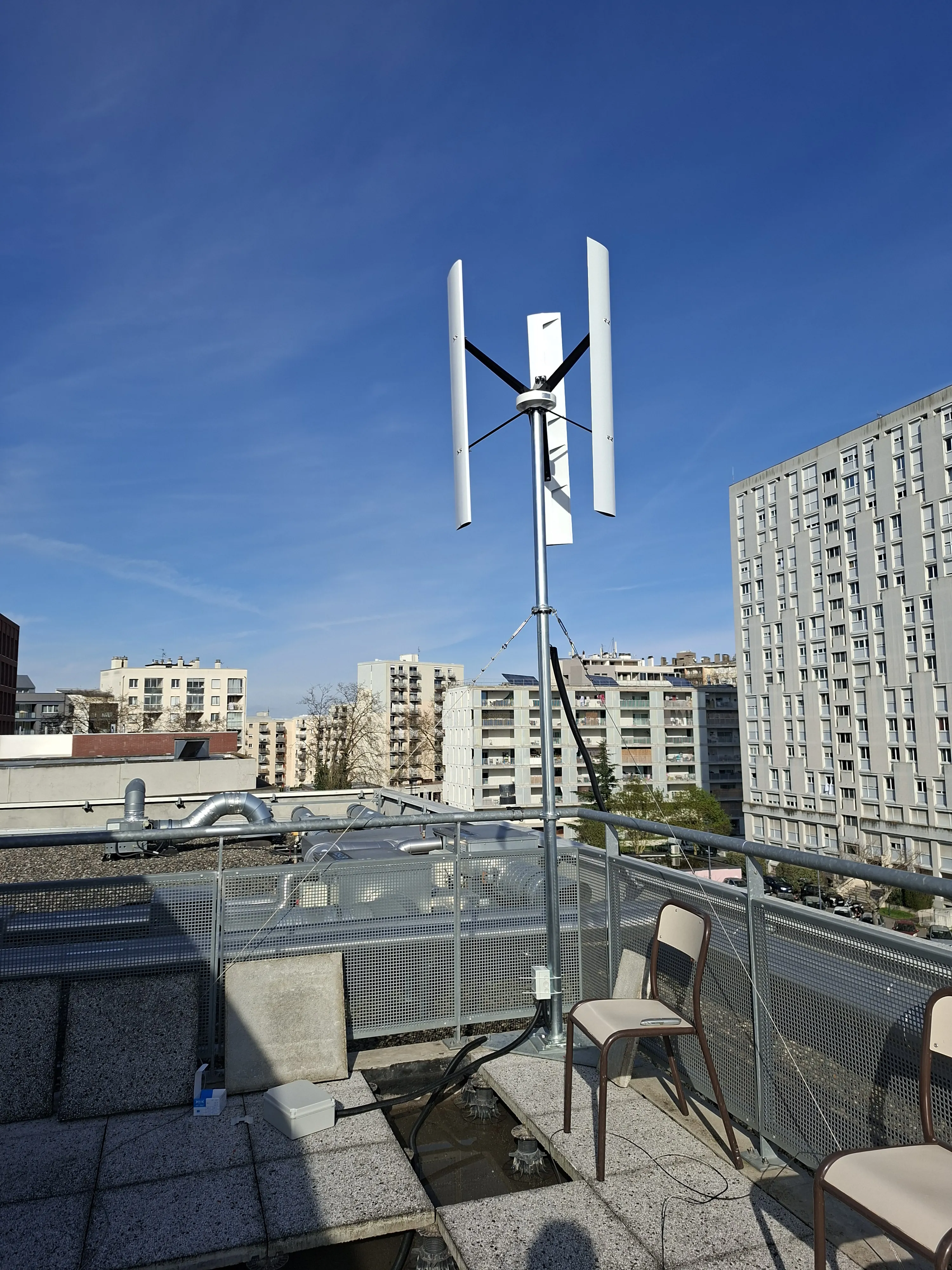
Cyril took the outdoor work. We inherited an existing PV canopy and had to make the rest of it a source the lab could use: batteries, wind, protection, drawings.

Storage on the roof is 9.6 kWh Li-ion. Wind is two vertical-axis machines, 1000 W and 800 W. Each turbine has its own cabinet for charge control.

The indoor bays

Four 19-inch bays. A typical stack, from the top: a 6 kW DC supply, a general e-stop, two Danfoss DC/AC converters, smart meters, LC filters, voltage/current sensors, L filters, extra current sensors, then protection and precharge at the bottom.

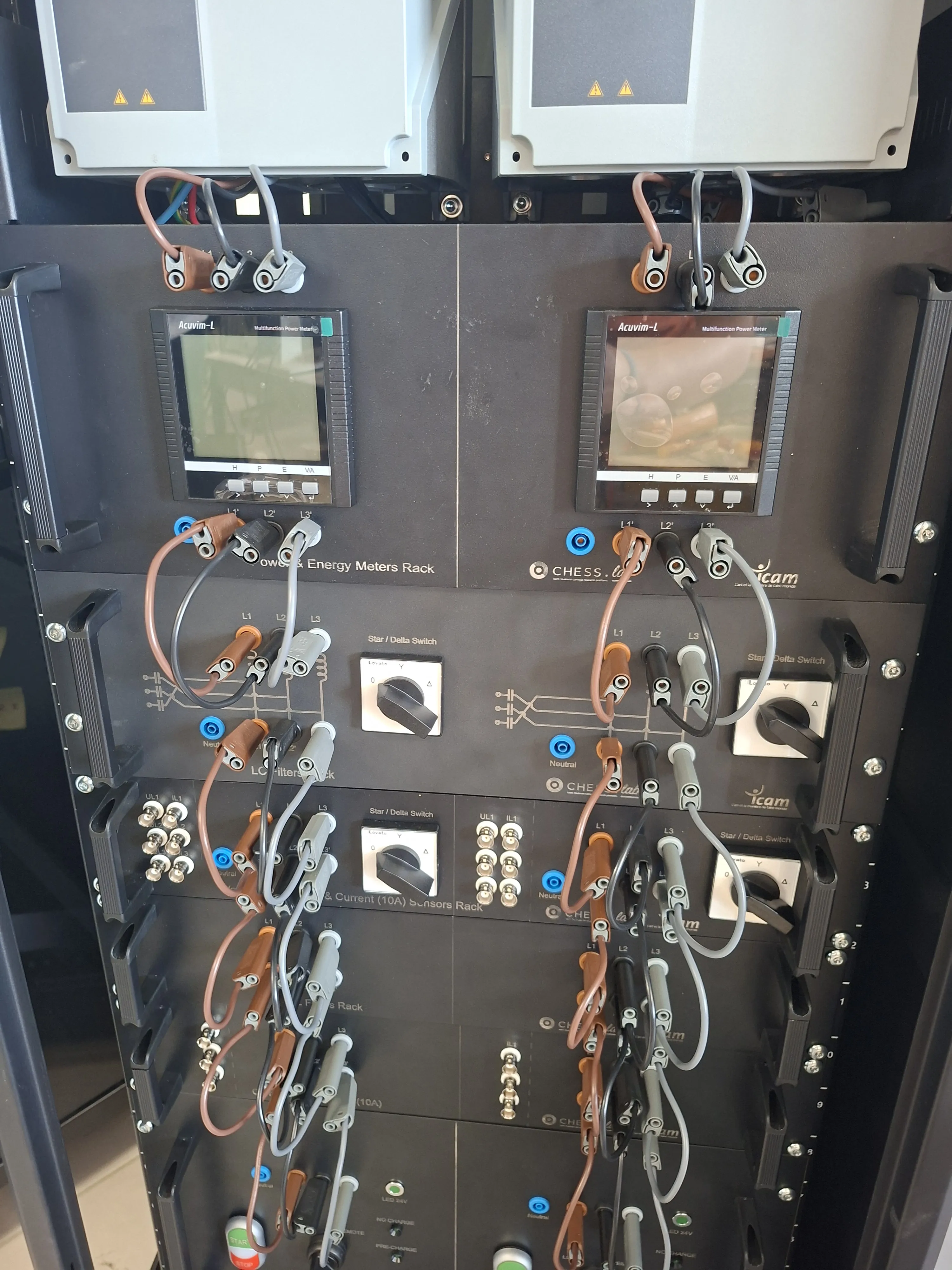
Finished 19-inch CHESS.lab racks: energy meters, L filters, voltage and current sensors, star-delta switches

The converters are industrial Danfoss VLT drives, used here as voltage-source inverters rather than motor drives. Two families: FC-302 and FC-202. The lab stock is 4 × 2.2 kW grid-forming and 8 × 1.5 kW grid-following. PWM and enable/reset come from the MicroLabBox, not from the Danfoss keypad.

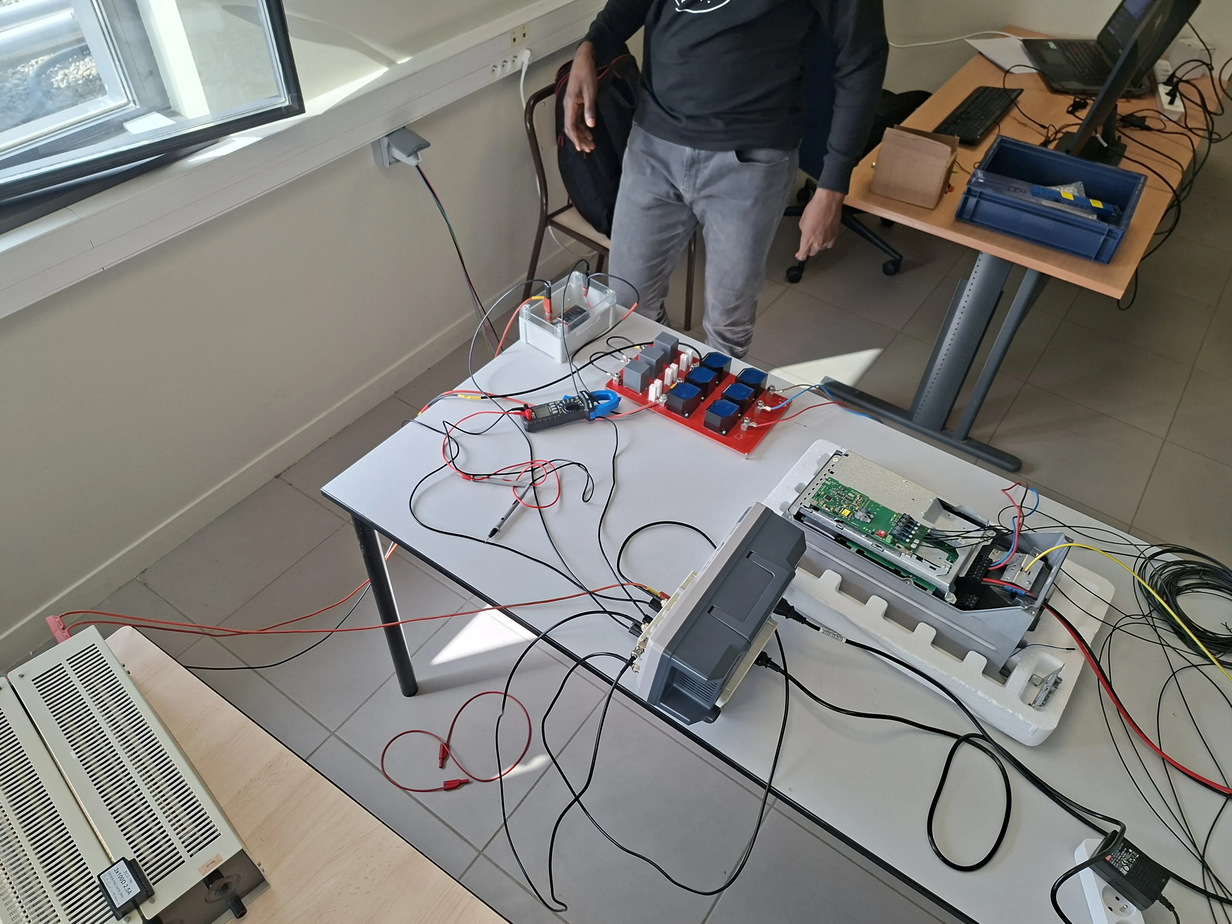
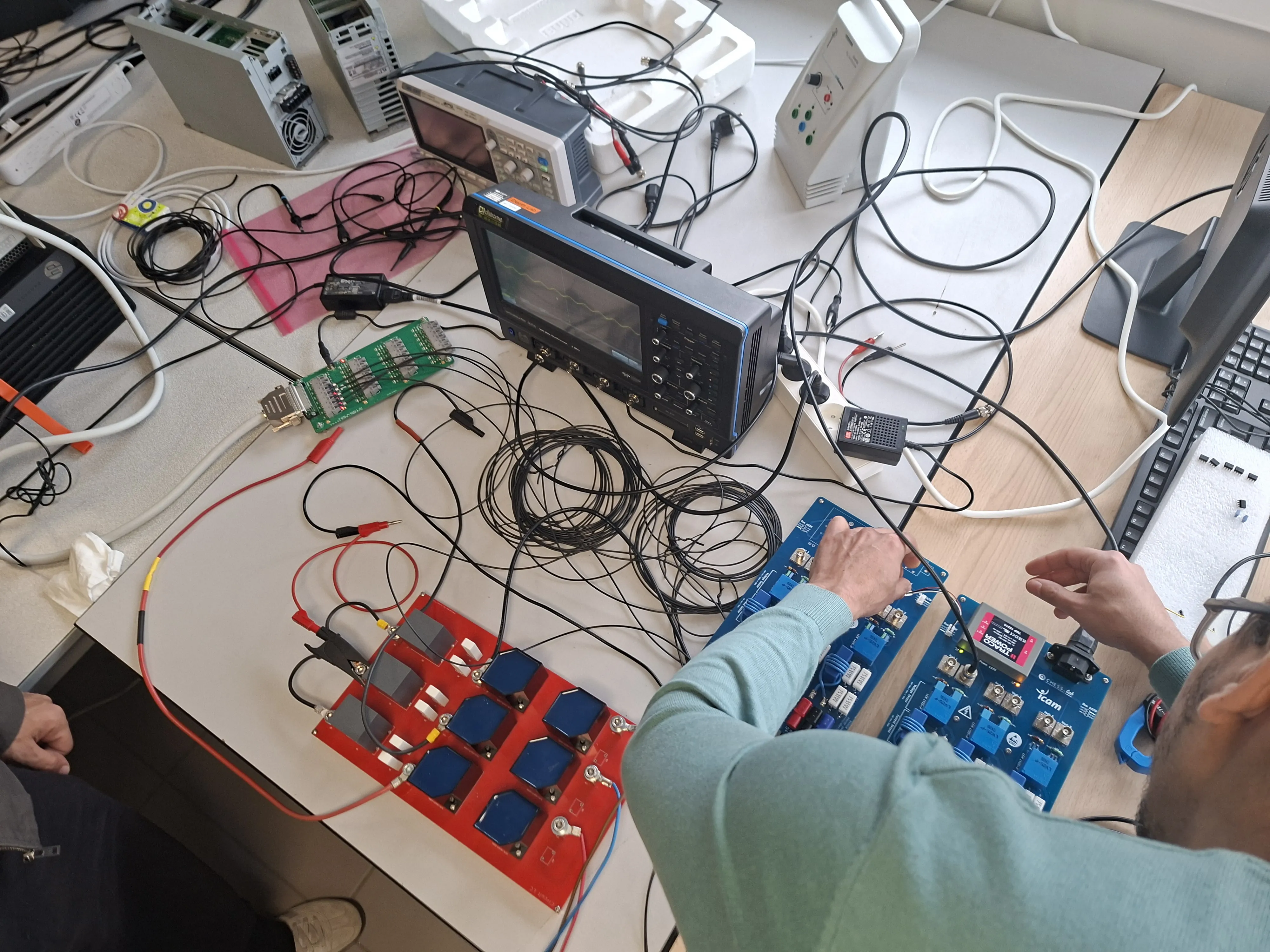
Opened Danfoss converter on the bench with a red LC-filter prototype and a DC supply

First weeks: take a drive apart, land PWM on the power stage, look at the chopped voltage on a scope. The red board on that table is an early LC filter. The grey brick is the converter with the cover off.

dSpace

The real-time box is a dSpace MicroLabBox II. Analog measurements come in on BNC. Digital lines can go out as PWM, enable and reset to the converters. ControlDesk is the interface: traces, setpoints, inverter configuration. Simulink is where the inner-loop models live. That chain is wired. We have not closed a current or voltage loop on the real inverters yet.

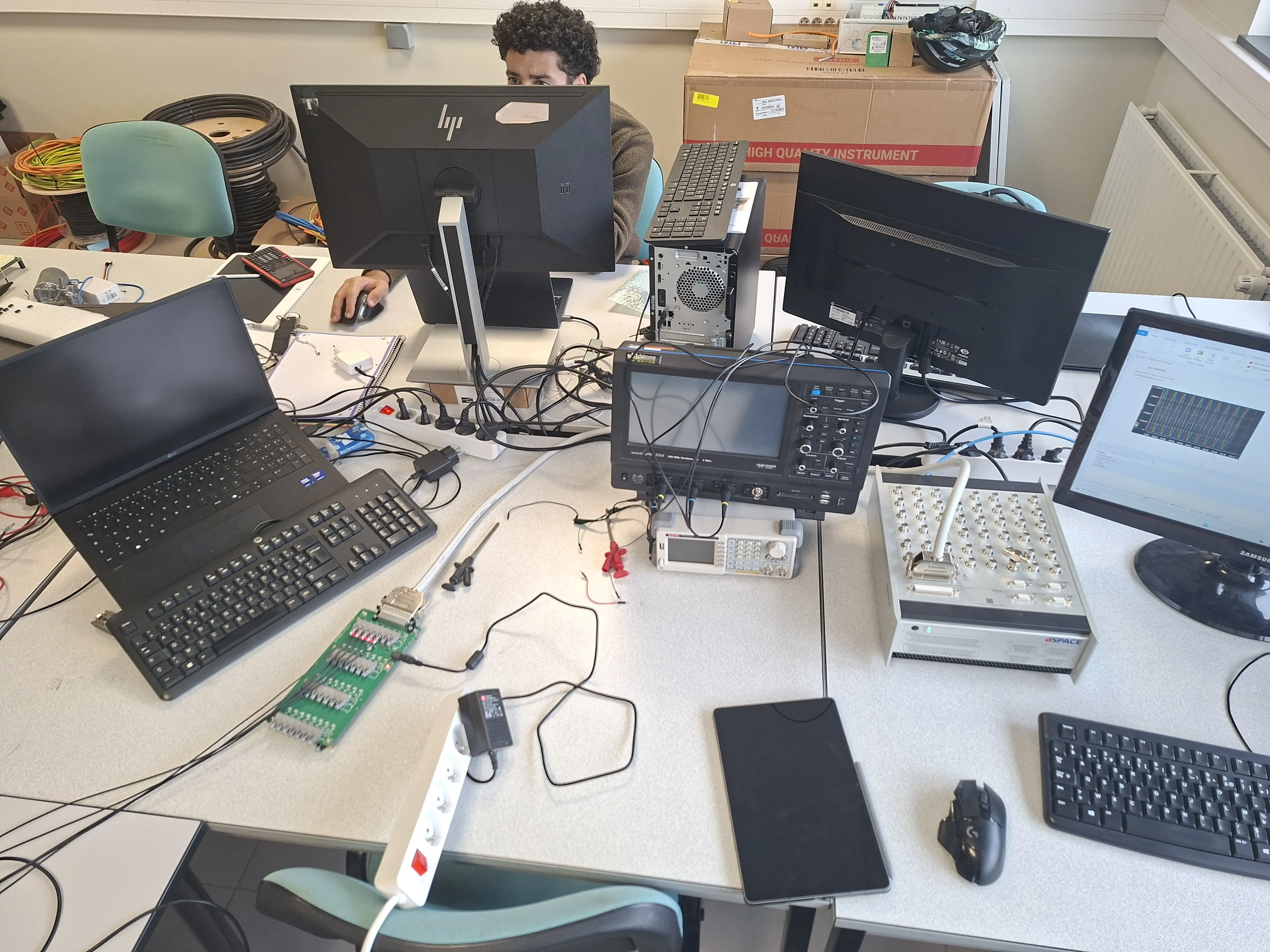
The commercial fibre interface from Aalborg (ipc2dspace-MLB, FC-X02 to dSpace) is 2750 €. We designed a plastic optical fibre board instead: 32 lines for four inverters, galvanic isolation, front-panel mount, about 300 €. Same job. That board sits between Simulink PWM and the Danfoss control card.

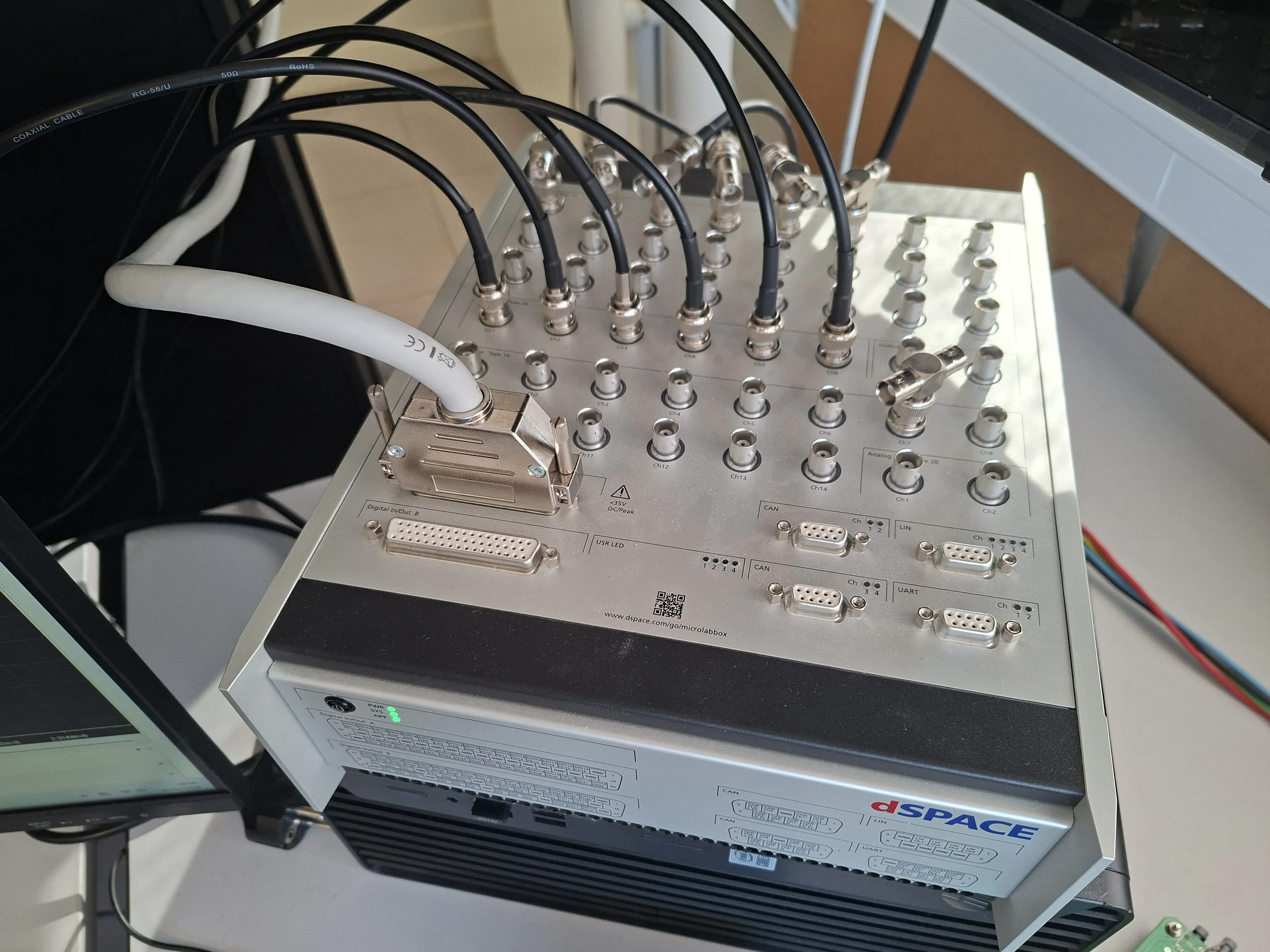
dSpace MicroLabBox II analog BNC inputs with coaxial cables

Coax, 50 Ω, into the analog bank. The box expects roughly ±10 V. The LEM boards sit upstream of those BNCs so a 400 V three-phase bus does not land on that front panel as 400 V. No extra conditioning stage in between: the MicroLabBox reads the sensor outputs directly.

LC filter

A VSI at 10 kHz is a square wave. The plant wants a sine. We sized an LC (then LCL) from the Kansas State and Aalborg references, then built our own.

Values on the board we assembled: Lf = 1 mH, Cf = 4.7 µF or 9 µF (switchable), Rcf = 3.3 Ω, Lc = 0.5 mH. Inductors are Schurter DLFL-0147-12D5, 12 A, 0.5 mH. Before the filter: 10 kHz commutation, high THD. After: a sine.

Teledyne LeCroy Wavesurfer 3054 showing three-phase voltages 120 degrees apart

Sensing

The sensor cards measure voltage and current at the filter output, isolated. They use LEM LV25-P for voltage and LEM LA55-P for current. The bench is sized for three-phase 400 V and 10 A. Current will not go beyond that.

LV25-P: primary is a current. For a 400 V line, peak with 5 % is 594 V. At 10 mA primary that wants R1 ≈ 59.4 kΩ. We used 60 kΩ as four 15 kΩ (E12). Measuring resistor Rm = 220 Ω.

LA55-P: 1:1000. For 10 A and a 3.5 V target, Rm calculates to 87.5 Ω. We used 82 Ω (E12). The first prototype boards were tested on the teaching benches before they went into a rack.

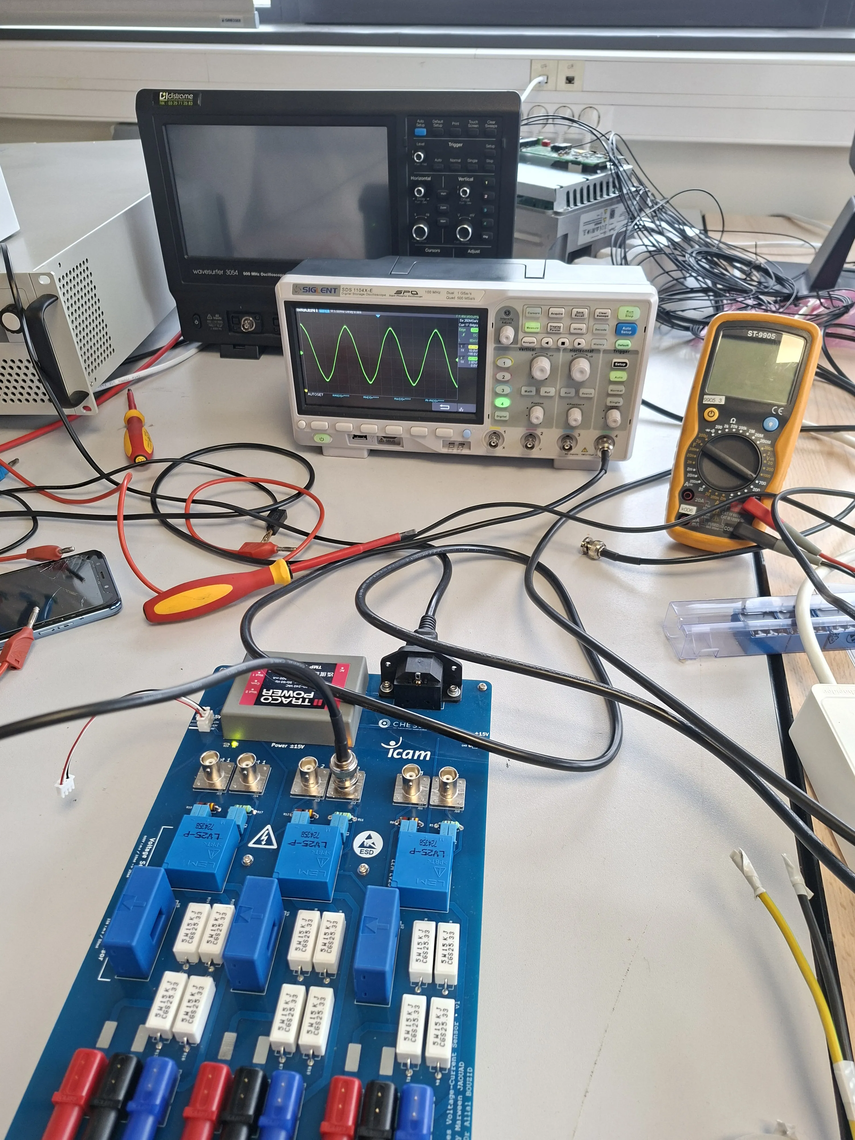
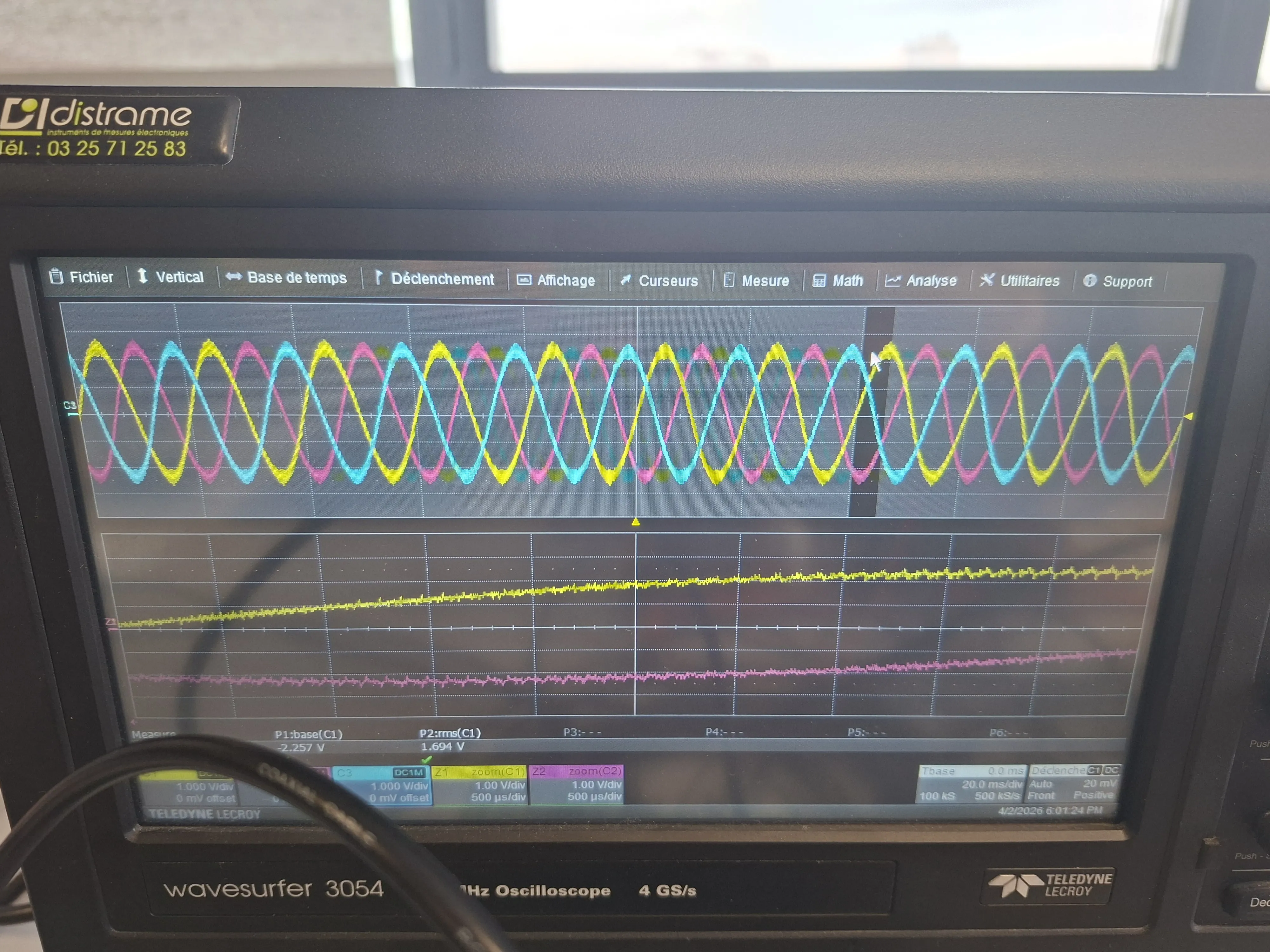
Icam voltage-current sensing PCB with LV25-P transducers, TRACO ±15 V module, and a sine on the scope

Blue Icam / CHESS.lab card, TRACO brick in the middle, LV25-P in blue, banana on the high-voltage side, BNC on the low-voltage side. The sine on the Siglent is the first evidence the divider and the LEM were in the right range.

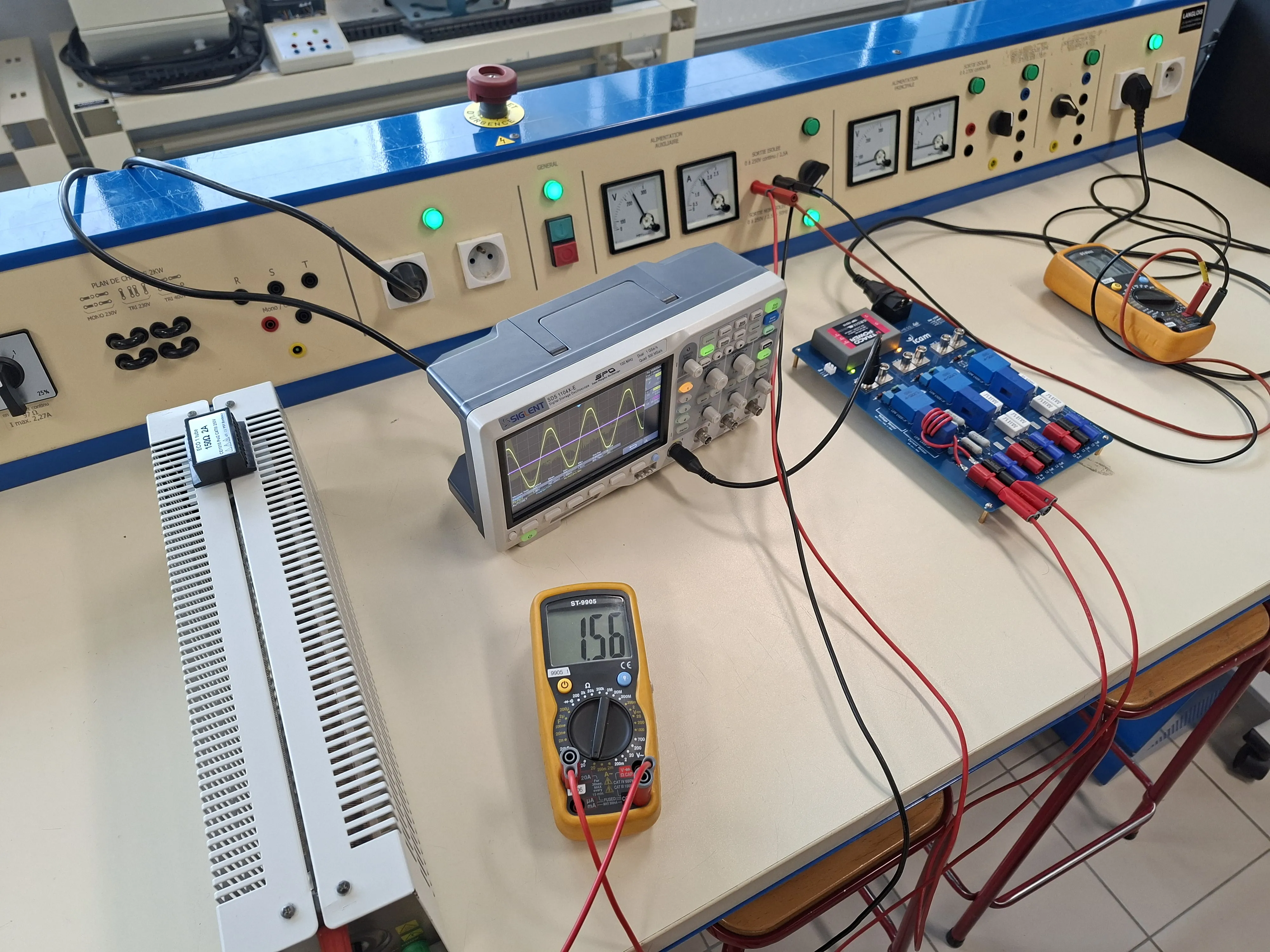
Sensing board on a teaching bench, three-phase sine on a Siglent scope, 15.6 V on the multimeter

Current-only cards sit in their own chassis: one box for two inverters, one for four, each with a TRACO TMP 30215. The 30215 takes 120 V to 370 V and puts out ±15 V at 1 A. Energy budget for 12 channels (6 voltage + 6 current), fans, LEDs, and the optional conditioning: 680 mA on +15 V and 430 mA on −15 V. 68 % and 43 % of the brick. That is why the supply is on the card and not a wall wart.

Conditioning (optional) and ground

With the MicroLabBox we do not use a conditioning stage. The LEM outputs already sit in a range the box can read. Conditioning is optional, for later, if we collect the same signals with an MCU: scale the amplitude, add offset for a unipolar ADC, anti-alias, clamp surges. The long 4-layer SMD card does that for six voltage and six current channels (TL084, buffer then inverting gain then summer). LTspice of one channel: sensor ±5.5 V, buffer, invert to ±1.65 V, sum into a 0 to 3.3 V window.

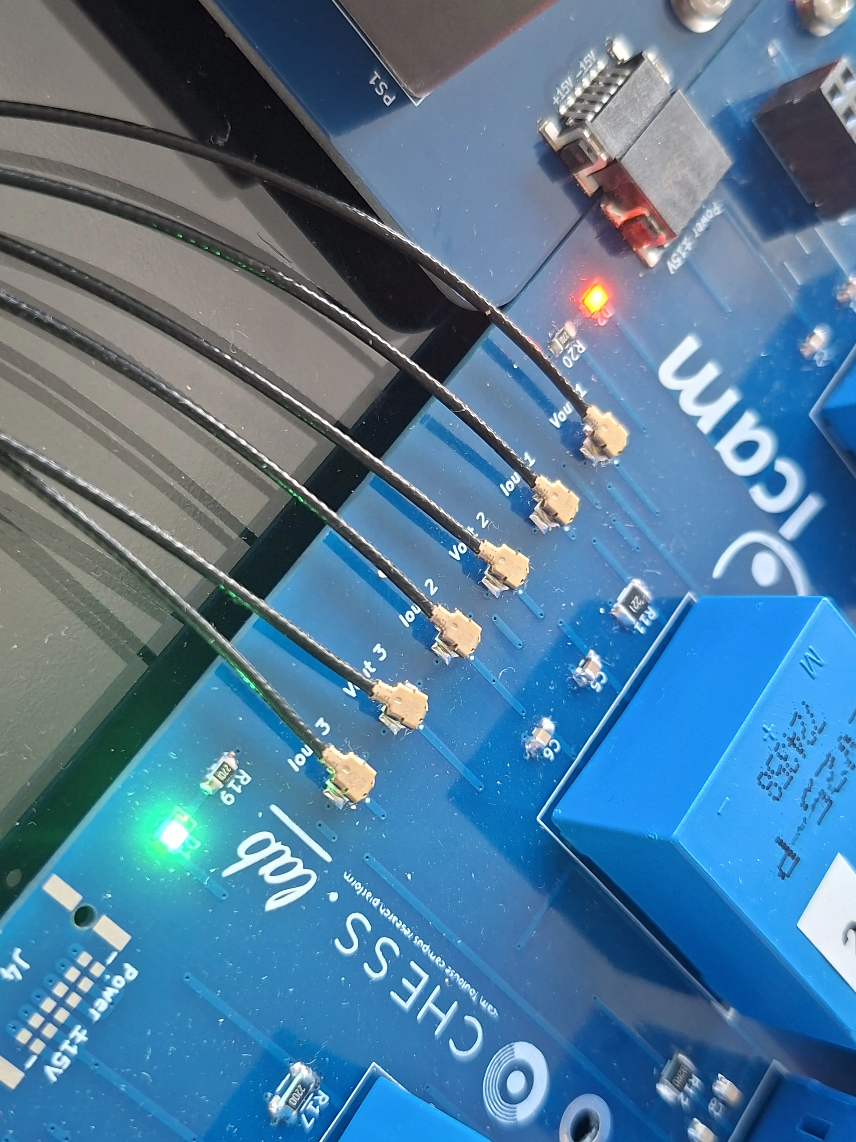
Ground is a star. Several chassis ties make a 50 Hz loop. One GND-to-chassis link, isolated BNCs on the front so the barrel does not become a second earth. Later sensor boards went smaller, SMD, supply off-board, standardised connectors. A commercial MTX1032-B is 782 €. The voltage-and-current board we built is about 200 €.

Close-up of MMCX coaxial outputs on the CHESS.lab sensing PCB, LV25-P and ±15 V

Racks

Choose the 19-inch chassis and the connectors (BNC, banana, rotary star/delta). Draw the front panels in SolidWorks. Send them out for engraving and cutting. Assemble: energy-meter rack (Acuvim-L), L-filter rack, voltage-and-current rack (10 A), the star/delta switch in the middle of the meter drawing.

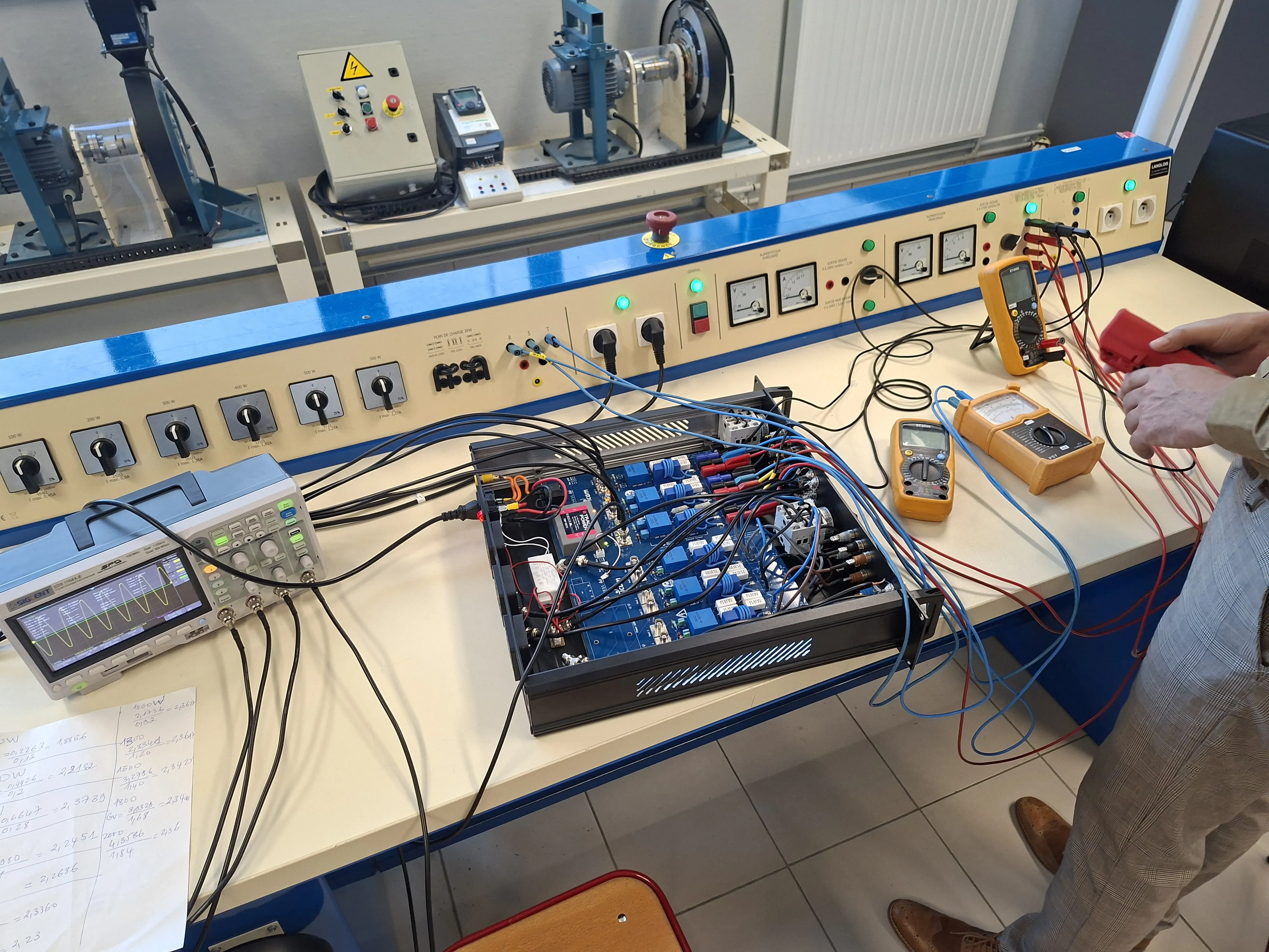
Voltage and current sensing boards in an open 19-inch chassis on a teaching bench, with gain calculations on paper

The point of the custom fronts is not cosmetics. Banana and BNC on the fascia mean you can rewire a test without opening the bay. Star/delta is a switch, not a recable. Compared with a commercial Imperix OP1300 at about 54 k€, the Icam bay sits around 20 k€: Danfoss converters, our sensors, our fibre, the MicroLabBox, the passives.

Simulink, inner loops

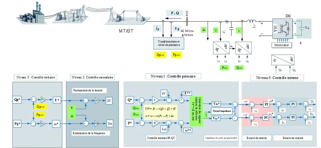
The usual microgrid stack has four levels (Julean, Aalborg 2009; Karn 2021 for the outer ones). We did not implement that stack. The diagram is the map. The Simulink work is only level 0: a current loop inside a voltage loop, in dq, on one distributed generator.

Level 0, inner. dq current loop inside a dq voltage loop, PWM to the VSI. This is the part in Simulink.
Level 1, primary. P-f / Q-V droop and a virtual impedance. Not in the model.
Level 2, secondary. Restore voltage and frequency. Not in the model.
Level 3, tertiary. Power setpoints against the upstream grid. Not in the model.

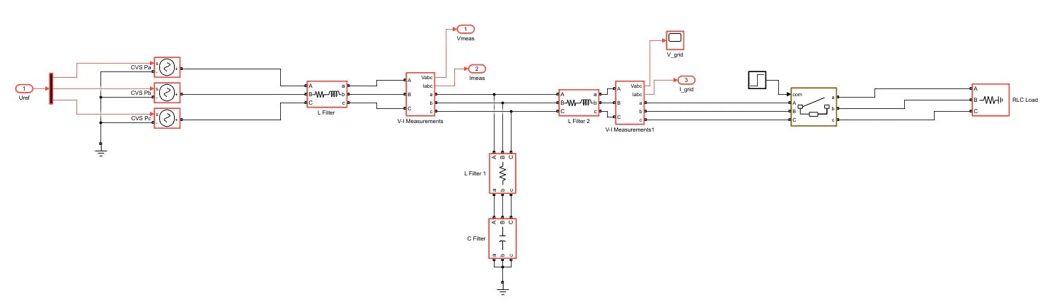
Four-level hierarchical control of a distributed generator. Only the inner loops were modelled.

The model is one inverter behind an LCL, with measurements and a breaker. An RLC load switches in at t = 0.5 s. Offline simulation on the PC, not running in real time on the MicroLabBox.

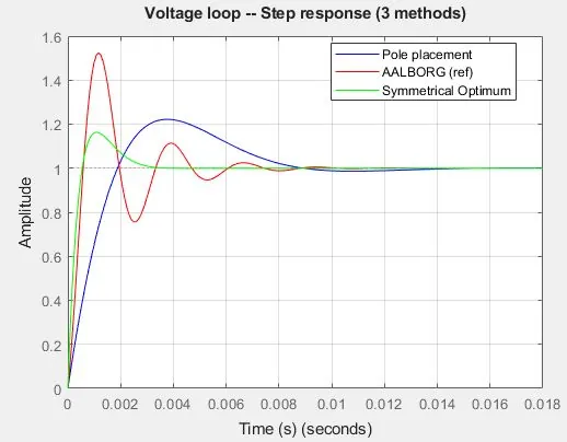
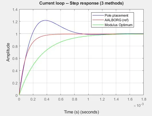
Simulink model of a distributed generator with LCL filter, measurements and a switched RLC load

For the inner PI I compared three tunings: pole placement, the Aalborg gains as a reference, and modulus / symmetrical optimum. Current loop, modulus optimum (the one we kept): Kp = 3.33 V/A, Ki = 253 V/(A·s), bandwidth 531 Hz. Voltage loop, symmetrical optimum: Kp = 0.030 A/V, Ki = 33.3 A/(V·s).

Voltage-loop step response for pole placement, Aalborg and symmetrical optimum

Current-loop step response for pole placement, Aalborg and modulus optimum

In that simulation, Vd is held at 325 V (peak of 230 V RMS). The load step at 0.5 s is a dip that recovers.

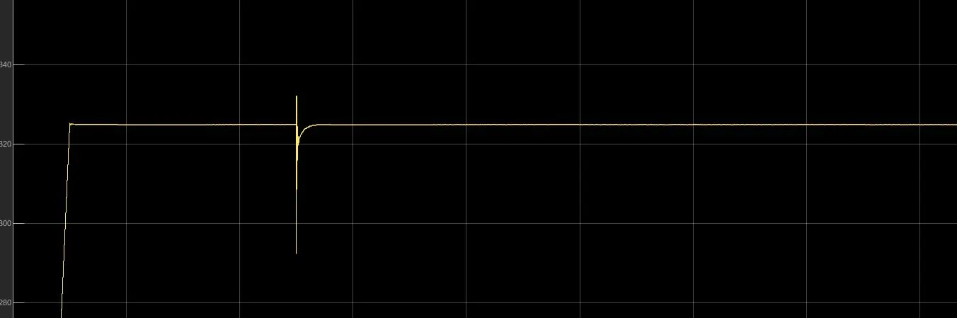
Simulink scope of Vd held at 325 V. No time axis is labelled; the dip is the 0.5 s load step.

The scope dump has no labelled time axis. Left to right is still time, and the dip in the middle of the window is that 0.5 s load step.

That is the simulation. Putting those loops on the MicroLabBox, then onto the Danfoss converters (grid-forming, grid-following, paralleling), is still ahead. Same for protection/precharge in the bay, and a few more boards (dSpace interface, Typhoon, an STM32/ESP32 microgrid PCB).

Topology wall

The indoor wall is ring, mesh and radial, switched with Crydom static relays. The idea: emulate line lengths, compare reliability and losses, watch power flow live. We pulled CIGRE LV line types (R, X, L) to pick L and R. Scaling those numbers as a true LV network was a dead end: systematic short-circuit, an X/R that does not behave, and no commercial LV line module that fits a rack. The workable path is to scale the network as MV, keep RLC consistent, and use off-the-shelf line inductors. The dynamics you care about stay; the bay does not eat itself.

The topology panel with protection still had to be finished. The drawing on the wall is the specification. The relays are the mechanism.

Budget and people

Semester envelope: 30 000 €. Spent: 29 841.56 €. Left: 158.44 €. Electronics 43.9 %, the indoor bays 29.9 %, outdoor equipment 15.6 %, topology panel 9.7 %, miscellaneous 1.0 %.