Hobby · January 2026

Comma.ai data visualization

With the precious help of Claude, I built a vehicle data visualization pipeline that fuses multiple sensor modalities into a real-time video overlay, similar to what Tesla FSD and Comma.ai's openpilot display. The goal was to understand how autonomous systems process and combine raw sensor data to make driving decisions.

Data source

I used the Comma2k19 dataset, an open-source collection of driving data captured by Comma.ai devices. The dataset includes multiple sensor streams: CAN bus data (vehicle speed, steering angle), GNSS positioning from both Qualcomm and u-blox receivers, IMU acceleration data, radar detections, and front-facing camera footage.

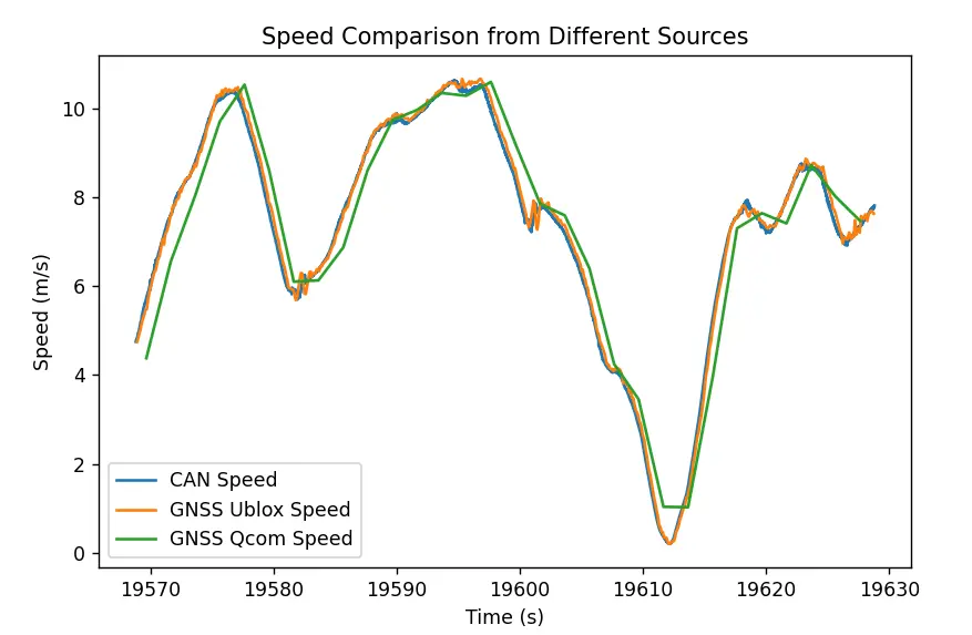
One of the first challenges was dealing with sampling rate differences: CAN data at 83Hz, GNSS u-blox at ~9.4Hz (vs 0.5Hz for Qualcomm), and video at 20fps.

Acceleration & speed

I started simple with a 60-second clip from a Toyota RAV4 driving through San Francisco (slow city driving, speed bumps, parked cars, red lights). To first understand the data structure, I began by working with acceleration from the IMU and speed from CAN. Then I plotted speed sources from CAN, GNSS Qualcomm, and GNSS u-blox. The u-blox proved much more precise with 561 data points vs only 30 from Qualcomm.

GPS mapping

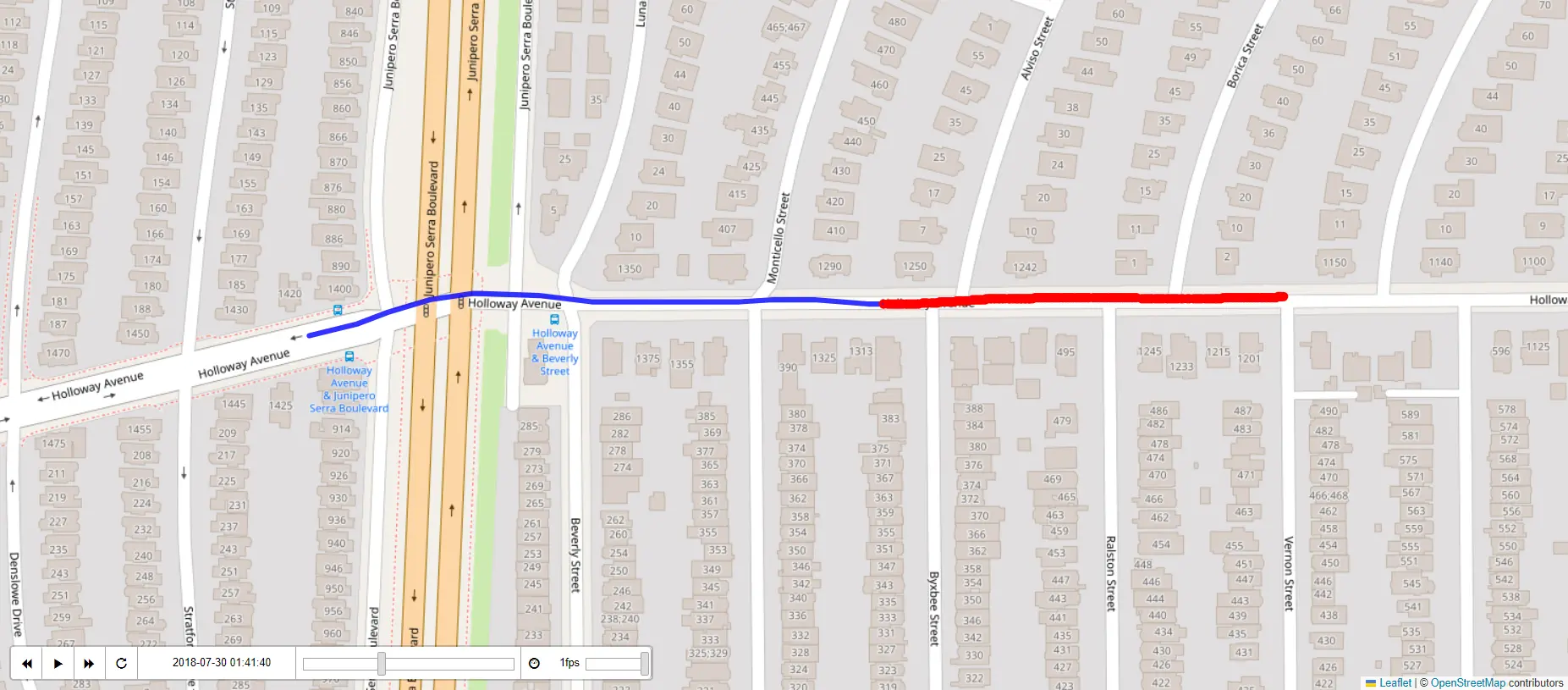
Using longitude and latitude data from the u-blox receiver, I built an interactive map visualization with Folium. The GNSS data was precise-enough that you could see exactly where the vehicle overtook the parked car. I added a slider to view the car's progress along its path.

Steering overlay

I extracted steering angle data from the CAN bus recording, which samples at 83Hz. To match the 20fps video, I downsampled and interpolated the data, then created a 60-second overlay showing the steering wheel position in real-time.

Lane detection

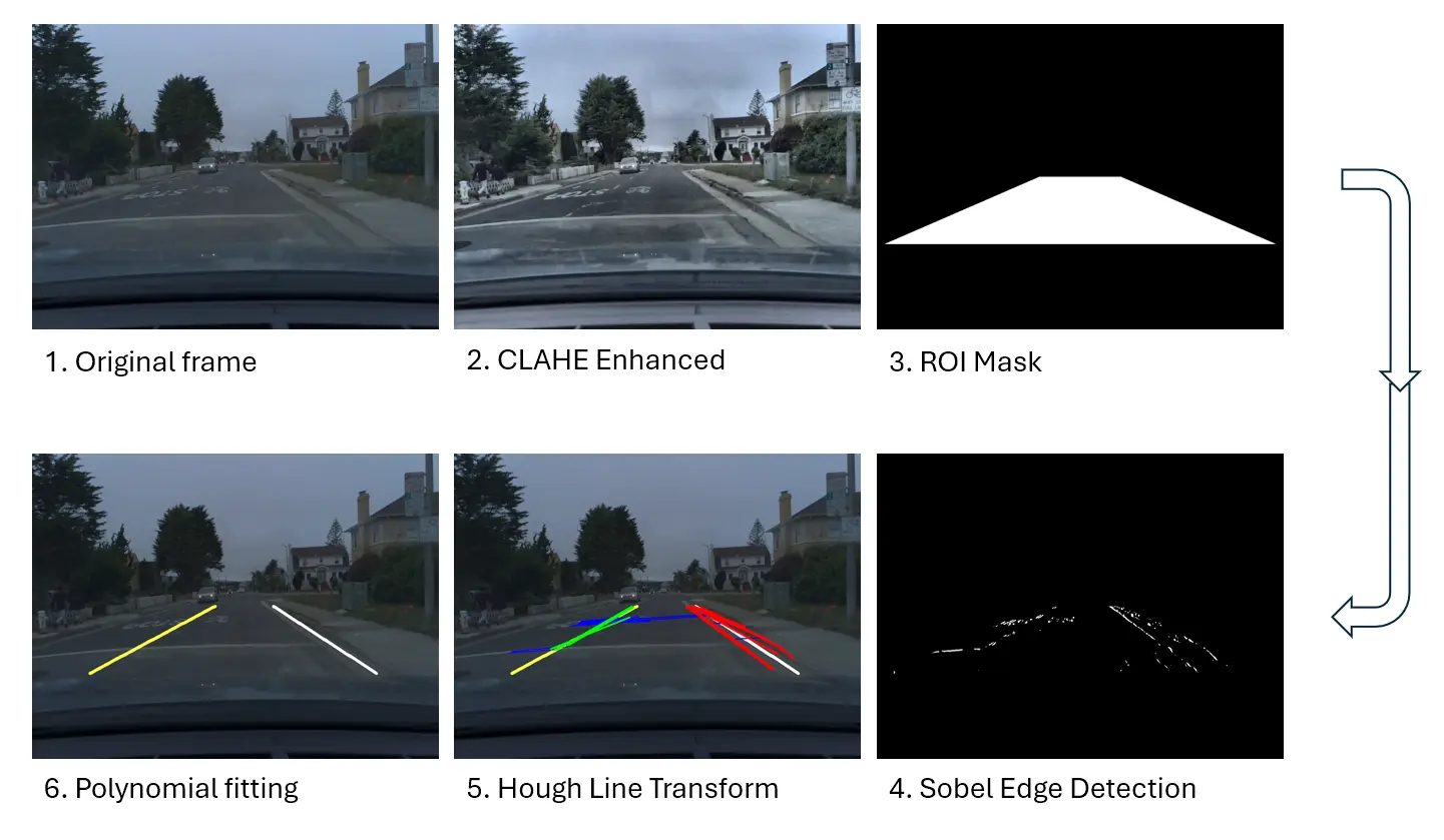
For lane detection, I initially tried DeepLabV3 but found that classical computer vision worked better for this use case. My pipeline combined CLAHE contrast enhancement, HSV/HLS color thresholding, Sobel edge detection for curb detection, Hough line transform for lane marking extraction, and Polynomial fitting. The approach worked well for straight roads, though intersections and curves remained challenging.

Depth estimation

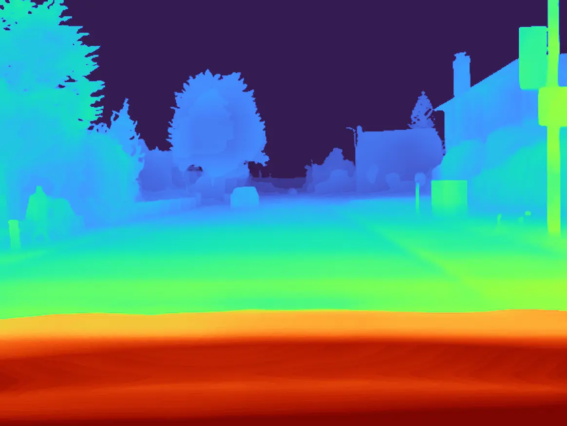
I used Depth Anything V2, a Vision Transformer model, for monocular depth estimation from the front camera. The output creates a heat map where blue represents far objects and red/yellow indicates close objects. This provides spatial understanding without requiring stereo cameras or LiDAR.

Object detection & radar fusion

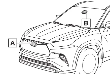
I combined YOLO object detection with radar detections using IoU-based (Intersection Over Union) matching. When a radar point overlaps with a YOLO bounding box, the match is shown in green, providing validated distance. Unmatched radar points appear in red. Due to the different placement between the radar (A) and the camera (B), an offset had to be accounted for. Most radar detection couldn't be matched with camera detections.

Path prediction

Using the steering angle and vehicle speed from CAN data, I implemented a bicycle model for path prediction. The model uses forward integration to predict the vehicle's trajectory, calculating slip angle with β = atan(lr/L × tan(δ)). This is the same kinematic model used in production autonomous vehicle systems.

Final integration

The final overlay combines all the components: vehicle speed from CAN, speed limits fetched via OpenStreetMap's Overpass API, a GPS mini-map with live position and heading, lane detection visualization (worse than thought), path prediction arc, and YOLO detections with distance estimates. The result looks similar to what Tesla FSD and Comma.ai's openpilot display.

Learnings

This project gave me hands-on experience with the core challenges of autonomous vehicle perception: time synchronization across sensors with different sampling rates, sensor fusion to combine complementary data sources, and the trade-offs between classical CV and deep learning approaches.